MATLAB tutorial

Everything You Always Wanted
to Know About `MATLAB`

but Were Afraid to Ask

Nicolas Aragon and Krzysztof Pytka

Istituto Universitario Europeo, Firenze
6 November 2013

MATLAB and other languages

MATLAB, R, Python

interpreted language
dynamic memory allocation

C, FORTRAN

compiled language
static memory allocation

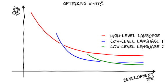
Shell commands

cd - change the working directory
pwd - print the current path
ls - list the working directory
exit - exit

Vectors and Matrices

Vectors


>> a=[1;2;3]
a =
     1
     2
     3

>> b=[1 2 3]
b =
     1     2     3

>> b'
ans =
     1
     2
     3

>> a+b
Error using  + 
Matrix dimensions must agree.
 
>> a+b'
ans =
     2
     4
     6

>> a*b
ans =
     1     2     3
     2     4     6
     3     6     9

>> b*a
ans =
    14

>> c=1:10
c =
     1     2     3     4     5     6     7     8     9    10

>>d=1:3:10
d =
     1     4     7    10

>> e=10:-2.5:1
e =
   10.0000    7.5000    5.0000    2.5000


>> linspace(3, 4.5, 5)
ans =

    3.0000    3.3750    3.7500    4.1250    4.5000

Matrices


>> A=[1 2 3; 4 5 6]    
A =

     1     2     3
     4     5     6

>> A(1,2)=3

A =

     1     3     3
     4     5     6

>> A(:,2)=[7,8]

A =

     1     7     3
     4     8     6


>> A(:)
ans =

     1
     4
     7
     8
     3
     6  

>> reshape(A, 3, 2)

ans =

     1     8
     4     3
     7     6


>> A=[1 2 3; 4 5 6];
>> A=[A; 7 8 9] %new row
A =
     1     2     3
     4     5     6
     7     8     9

>> A=[1 2 3; 4 5 6];
>> A=[A [1;1]] %new column
A =
     1     2     3     1
     4     5     6     1

Matrix operations vs. array operations



>> A=[1 2; 3 4];
>> A*A

ans =

     7    10
    15    22

>> A.*A

ans =

     1     4
     9    16

>> A^2

ans =

     7    10
    15    22

>> A.^2

ans =

     1     4
     9    16

Construction of Matrices


>> A=zeros(2,3)
A =

     0     0     0
     0     0     0

>> B=ones(2,3)
B =

     1     1     1
     1     1     1

>> C=eye(4)
C =

     1     0     0     0
     0     1     0     0
     0     0     1     0
     0     0     0     1

>> diag(eye(3))
ans =

     1
     1
     1
     

>> diag([1 2 3])
ans =

     1     0     0
     0     2     0
     0     0     3

Random numbers


>> A=rand(3,2)

A =

    0.1419    0.7922
    0.4218    0.9595
    0.9157    0.6557

>> B=randn(3,2)

B =

   -1.2075    0.4889
    0.7172    1.0347
    1.6302    0.7269

>> C=randi([-100 100], 3,2)

C =

   -91    39
   -81   -37
    65    90

>> D=floor(rand(3,2)*201-100)

D =

    -1    43
   -10    52
    30   -44

Dimension-reducing functions


>> A=rand(5,2)
A =
    0.5215    0.9121
    0.9954    0.6560
    0.8998    0.9232
    0.7072    0.6794
    0.0199    0.1271

>> sum(A)
ans =
    3.1438    3.2978    

>> max(A)
ans =
    0.9954    0.9232

>> mean(A)
ans =
    0.6288    0.6596




>> corrcoef(A)
ans =
    1.0000    0.7394
    0.7394    1.0000

Non-standard normal distribution(Example)

Draw sample of $10^5$ observations from distribution given by $\left(\substack{y_1\\y_2}\right)\sim \mathcal{N} \left( \left(\substack{2\\1}\right), \left[ \begin{array}{cc} .75 & .1 \\ .1 & .25 \\ \end{array} \right]\right).$

Hint:

We know that if $x\sim \mathcal{N}(\mu, \Sigma) $ and $y=\alpha+B x,$ then $y\sim\mathcal{N}(\alpha+B \mu, B \Sigma B').$ Given $ x\sim \mathcal{N}(0, \mathbf{I}),$ we can produce $y$ by transformation $y=\left(\substack{2\\1}\right)+Bx,$ where $B$ is a Cholesky decomposition of $\mathbf{\Sigma}=\left[ \begin{array}{cc} .75 & .1 \\ .1 & .25 \\ \end{array} \right]$ such that $chol\left(\mathbf{\Sigma}\right)=BB'.$

Non-standard normal distribution(Example)

Solution


>> X=randn(2, 1e5);
>> mean(X')
ans =
   -0.0048    0.0098

>> std(X')
ans =
    0.9996    0.9991

>> d=[.75 .1; .1 .25];
>> d=chol(d, 'lower')
d =
    0.8660         0
    0.1155    0.4865



>> Y=d*X+repmat([2;1], 1, 1e5);
>> cov(Y')
ans =

    0.7504    0.0991
    0.0991    0.2489

>> mean(Y')
ans =
    2.0004    0.9980

Conditional statements

`if/elseif/else`



if [expr1]
  [sth1] %do if expr1

elseif [expr2]
  [sth2] %do if expr2 and not expr1

else
  [sth3] %do if not expr1 and not expr1
end

Relational and logical operators

== - equal
< - less than
<= - less than or equal
~= - not equal
> - greater than
>= - greater or equal
&& - short-circuit logical AND
|| - short-circuit logical OR

Random Economist Generator (Example)

Write a program which draws string 'Debreu' with a probability of .5, 'Sargent' with a probability of .3, and 'Lange' with a probability of .2.


x=rand(1)

if x<.5
    x='Debreu'
elseif x<.8 % why don't we have to check if x>.5?
    x='Sargent' 
else
    x='Lange'
end;

Loops

`for`


for i = 1:100
    disp('I will hand in macro problem sets on time...') 
end

Waitbar


h = waitbar(0,'Please wait...'); %initialize a waitbar
steps = 1000;
for step = 1:steps
    pause(.1)
    waitbar(step / steps) %updata the waitbar
end
close(h) %close the waitbar

Probability of range(Example)

Let $x\sim\mathcal{N}(0,1).$ Compute numerically:

$P(|x|<1),$
$P(-\frac{1}{2}< x<1).$


N=1e7;
x=randn(N,1);

counter=0
for i=1:length(x)
    if abs(x(i))<1
        counter=counter+1;
    end
end;
frac1=counter/N;
frac1

%%%

counter=0
for i=1:length(x)
    if x(i)<1 && x(i)>-.5
        counter=counter+1;
    end
end;
frac2=counter/N;
frac2

`while`

But what if we don't know a number of iterations?


count=1;
x=0
while x>=0
    
    ['x has been non-negative for  ', num2str(count), ' iterations']
    x=randn(1)
    count=count+1;
    
end;

Plotting

Plots


X=randn(30,1)
y=rand(1)*X+randn(30,1);
plot(X,y, 'p')
xlabel('X')
ylabel('y')
title('Title')
legend('X')
grid()

X=randn(30, 6);
alpha=[1 2.5 -10 100 -100 0]';
y=X*alpha+randn(30,1);
for i=1:6
    subplot(3,2,i)
    plot(X(:,i), y, 'p')
    grid()
    
end;


X=randn(30,1);
alpha=[10 -10];
y=X*alpha+randn(30,2);
plot(X, y, 'x')
legend('positive', 'negative')
grid()

Histograms


X=randn(300,1)

hist(X)
grid()

hist(X,100)

Functions


function [mean,stdev] = stat(x)
            %STAT Interesting statistics.
            n = length(x);
            mean = sum(x) / n;
            stdev = sqrt(sum((x - mean).^2)/n);
        end


A=rand(10,1);
[meanA,stdA]=stat(A); %both outputs
meanA=stat(A); %1st output only
[~,stdA]=star(A); %2nd output only

`OLS.m` file:


function beta=OLS(X,y)
    
    beta=inv(X'*X)*X'*y;
end

`ridge.m` file:


function beta=ridge(X,y, lambda)
    s=size(X);
    beta=inv(X'*X+lambda*eye(s(2)))*X'*y;
end

Scope of variables

`sum_n.m`


function result=sum_n(input)
    result=sum(input(1:N));
end

Command Window


>> X=randn(300,1);
>> N=100;
>> sum_n(X)

Undefined function or variable 'N'.

Error in sum_n (line 3)
    result=sum(input(1:N))

Global variables

`sum_n.m`


function result=sum_n(input)
    global N;
    result=sum(input(1:N));
end

Command Window


>> X=randn(300,1);
>> global N;
>> N=100;
>> sum_n(X)
ans =
   10.0110

Using global variables is not good practice!

source: xkcd.com

Using new input is better

`sum_n.m`


function result=sum_n(input, k)
    
    result=sum(input(1:k));
end

Command Window


>> X=randn(300,1);
>> N=100;
>> sum_n(X,N)
ans =
  -11.3050

Memory Preallocation

(Example)

Let $y_t\in \mathbb{R}^{200}$ be governed by a law of motion $y_{t+1}=A\cdot y_t$. Given $y_0$ and $A\in \mathcal{M}_{200\times 200},$ please replicate dynamics of the system for a horizon of 100 periods.


A=randn(200,200);
y1=randn(200,1);
y2=zeros(200,100);
y2(:,1)=y1;

tic;
for i=2:100
    y1(:,i)=A*y1(:,i-1);
end;
time1=toc;

tic;
for i=2:100
    y2(:,i)=A*y2(:,i-1);
end;
time2=toc;

['Wow! Simple preallocation speeds up the computation ' num2str(time1/time2) ' times!!!']

sum(sum(y1~=y2)') %what is it for?

Ridge vs. OLS (Example)

Please, compare statistical properties of OLS and Ridge regression using simulations.


rng(50524)
n_par=2
X=[ones(100,1),randn(100,n_par-1)] %first column: common intercept; the remaining covariates
par=randn(n_par,1)

y=X*par+randn(100,1)

for i=1:min(n_par,6)
    subplot(3,2,i)
    plot( X(:,i),y, 'p')
    xlabel(strcat('regressor ', num2str(i)))
end;




N=1e4;
beta_ols=zeros(N,n_par);
beta_ridge=beta_ols;
h=waitbar(0, 'Initializing the waitbar?');

for i=1:N
    y=X*par+5*randn(100,1);
    beta_ols(i,:)=OLS(X,y)';
    beta_ridge(i,:)=ridge(X,y, 3.5)';
    
    waitbar(i/N, h, sprintf('%d%% along...',round(i/N*100)))
end

close(h)
subplot(2,1,1)
hist(beta_ols(:,2))
subplot(2,1,2)
hist(beta_ridge(:,2))

Everything You Always Wanted to Know About MATLAB

but Were Afraid to Ask

Table of Contents

MATLAB and other languages

MATLAB, R, Python

C, FORTRAN

Shell commands

Vectors and Matrices

Vectors

Matrices

Matrix operations vs. array operations

Construction of Matrices

Random numbers

Dimension-reducing functions

Non-standard normal distribution(Example)

Hint:

Non-standard normal distribution(Example)

Solution

Conditional statements

if/elseif/else

Relational and logical operators

Random Economist Generator (Example)

Loops

for

Waitbar

Probability of range(Example)

while

Plotting

Plots

Histograms

Functions

Functions

OLS.m file:

ridge.m file:

Scope of variables

sum_n.m

Command Window

Global variables

sum_n.m

Command Window

Using global variables is not good practice!

Using new input is better

sum_n.m

Command Window

Memory Preallocation

(Example)

Ridge vs. OLS (Example)

Everything You Always Wanted
to Know About `MATLAB`

`if/elseif/else`

`for`

`while`

`OLS.m` file:

`ridge.m` file:

`sum_n.m`

`sum_n.m`

`sum_n.m`